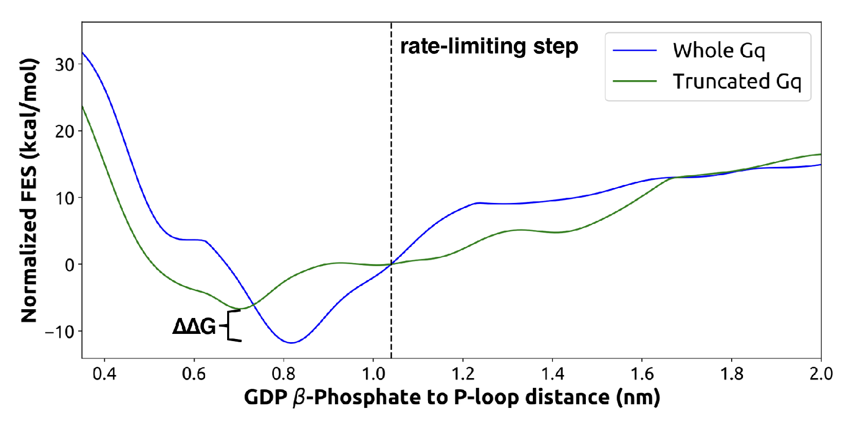
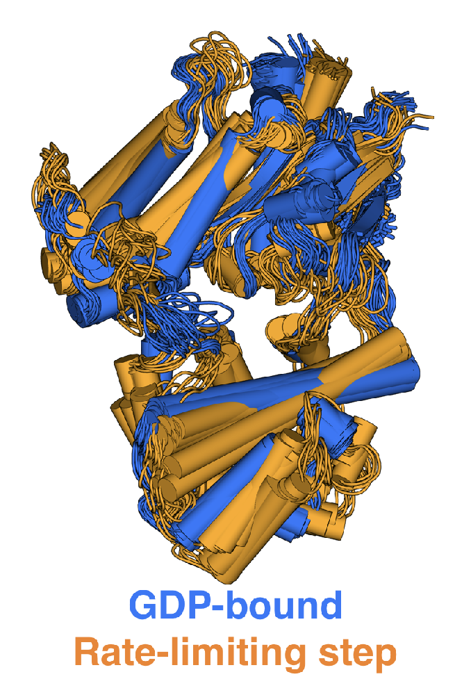
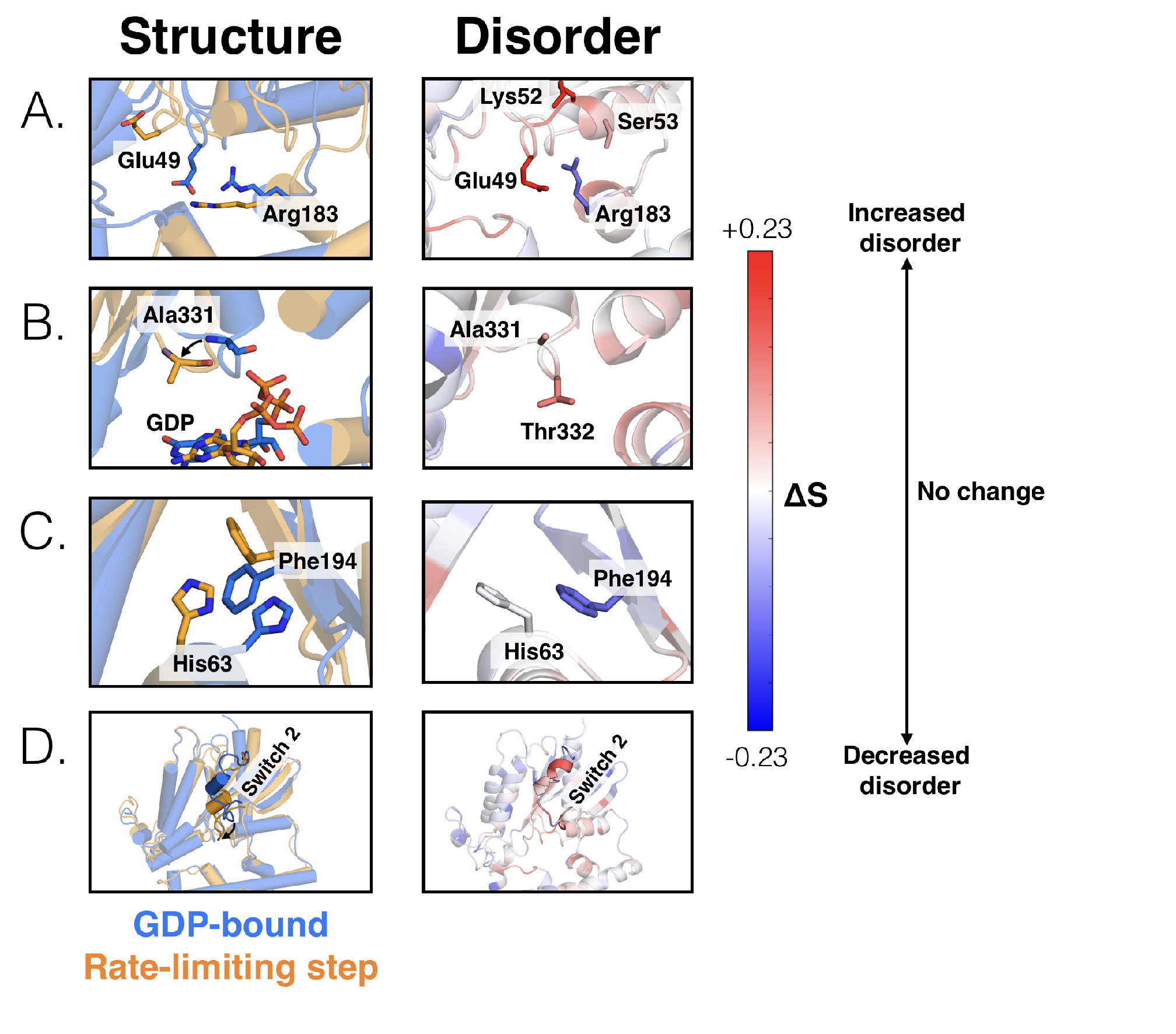
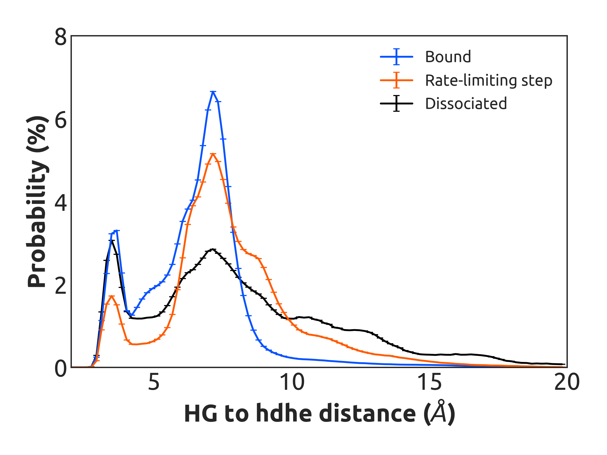
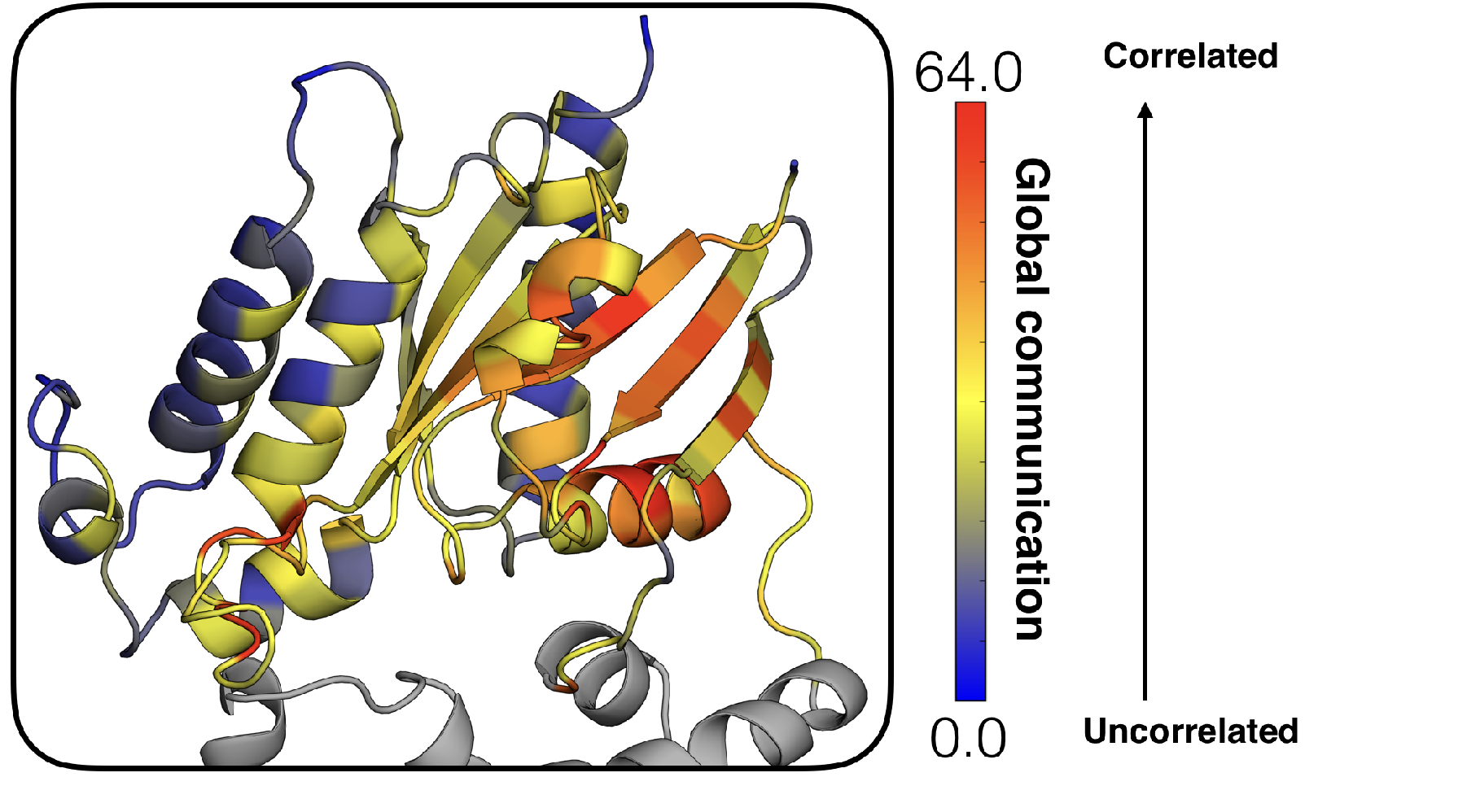
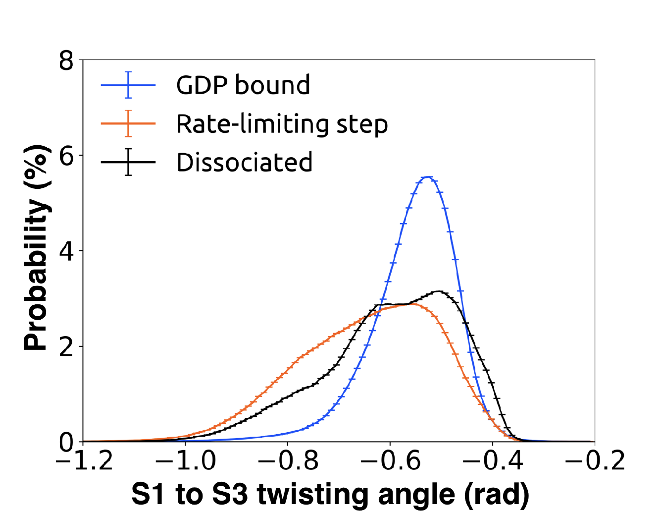
B Supplementary figures highlighting the mechanism of GDP release

Appendix B
Supplementary figures highlighting the mechanism of GDP release

The work in this Appendix is published in: SSun, X. $^{*}$ and Singh, S. $^{*}$ , Blumer, K.J., and Bowman, G.R., Simulation of spontaneous G protein activation reveals a new intermediate driving GDP unbinding. eLife, 7, October 2018, https://doi.org/10.7554/eLife.38465.001 [48]

B.1 Supplementary Figures

Figure B.1: Free-energy surface from metadynamics simulations of GDP release for the full G

α

q (blue) and truncated form (green, without the last five C-terminal residues). Both sets of simulations were run for the same amount of time with identical collective variables. The rate-limiting step as identified from the highest flux pathway is marked with a dashed line. The free-energy difference between the GDP-bound states of the two systems is marked with a bracket.

Figure B.2: Overlay of representative structures of G

α

q when bound to GDP (blue) or across the rate-limiting step (orange).

Figure B.3: Changes in the structure (left) and disorder (right) of specific regions across the rate-limiting step. (A) Residues that contact the phosphates of GDP, including the salt bridge between Glu49

^{G . s 1 h 1.4}

and Arg183

^{G . h f s 2.2}

, (B) the s6h5 loop, (C) the

π - π

stacking interaction between Phe194

^{G . S 2.6}

and His63

^{G . H 1.12}

, and (D) switch 2.

Figure B.4: Distribution of distances between the side-chains of K275

^{G . s 5 h g . 1}

and D155

^{H . h d h e . 5}

for the GDP-bound state (blue), across the rate-limiting step (orange), and upon GDP dissociation (black).

Figure B.5: Implied timescales for the Markov state model. (A) Top 10 implied timescales for the 5040 states of G

α

. (B) Top 10 implied timescales for the final 221965 states.

Figure B.6: Probability distribution of the distance between Leu349

^{G . H 5.16}

on H5 and Phe194

^{G . S 2.6}

on S2 to monitor the tilting motion of H5 upon GDP release when bound to GDP (blue), across the rate-limiting step (orange), and upon GDP dissociation (black). In the GDP bound state (blue), such a distance is peaked at 15 Å. Across the rate-limiting step (orange), tilting motion of H5 upon GDP release occurs with a peak in distance at 12.5 Å.

Figure B.7: H5 vertical motion is sampled across GDP release simulations. At each point, the combined population (represented by the color scale) of that state is shown using both GDP-bound and intermediate stages of the GDP release pathway. H5 vertical motion was measured by computing the distance between Thr334

^{G . H 5.1}

on the s6h5 loop and Phe341

^{G . H 5.8}

on H5. GDP release distance was measured as the distance from GDP

β

-phosphate to the center of mass between residues Lys52

^{G . H 1.1}

, Ser53

^{G . H 1.2}

, and Thr54

^{G . H 1.3}

on H1.

Table B.1: Measurements comparing tilting and translation of H5 across PDB structures and MD simulation.

Construct description

PDB ID

H5 Tilting

Distance (Å)

H5 Vertical

translation distance (Å)

H5 Tilting

residues used

H5 Translation

residues used

α

q-GDP

3AH8

13.5

10.6

Tyr325 to Leu349

Thr334 to Phe341

α

q after rate

limiting step from MD

N/A

15.1

11.1

Tyr325 to Leu349

Thr334 to Phe341

α

i-GDP

1GP2

10.3

10.2

Tyr320 to Ile343

Thr329 to Phe336

α

i-µOR

6DDF

14.6

13.0

Tyr320 to Ile343

Thr329 to Phe336

α

i-A1AR

6D9H

13.8

10.1

Tyr321 to Ile344

Thr330 to Phe327

α

i-Rhodopsin

6CMO

15.8

10.7

Tyr320 to Ile343

Thr329 to Phe336

α

o-5HT1B

6G79

13.1

14.2

Tyr310 to Ile333

Thr319 to Phe326

α

s-B2AR

3SN6

12.8

14.6

Tyr360 to Ile383

Thr369 to Phe376

Figure B.8: Allosteric network connecting hNs1 contacts to the P-loop and switch 1 via S4. CARDS data showing communication per residue to a target site (dashed box) is plotted (left) and mapped onto the structure of G

α

q (right) for (A) hNs1, (B) S1 (C) S4 (D) the P-loop and (E) Switch 1. Arrows indicate important regions with significant communication to the target site.

Figure B.9: Global communication of each residue in the Ras-like domain mapped onto the structure of G

α

q, colored based on the scale (right). The helical domain (gray) is shown for orientation.

Figure B.10: Probability distributions of the twist angle between S1 and S3. The dihedral angle is computed by taking the dihedral angle between the CA atoms of Leu45

^{G . S 1.7}

, Leu40

^{G . S 1.2}

, Val199

^{G . S 3.1}

, and Asp205

^{G . S 3.7}

, so that the angle measured represents S1/S3 twisting at the GPCR facing side. Twist was computed for GDP bound(blue), intermediate(orange), and GDP dissociated states(black).

[next] [prev] [prev-tail] [front] [up]

Appendix BSupplementary figures highlighting the mechanism of GDP release

B.1 Supplementary Figures

Appendix B
Supplementary figures highlighting the mechanism of GDP release